Welcome to metocean-stats’s documentation!
metocean-stats is a Python package (under developement) for metocean analysis of NORA3 (wind and wave) hindcast.
- The package contains functions that:
generate statistics (tables, diagrams etc)
Installing metocean-stats
Alternative 1: Using Mambaforge (alternative to Miniconda)
Install mambaforge (download)
Set up a Python 3 environment for metocean-stats and install metocean-stats
$ mamba create -n metocean-stats python=3 metocean-stats
$ conda activate metocean-stats
Alternative 2: Using Mambaforge (alternative to Miniconda) and Git
Install mambaforge (download)
Clone metocean-stats:
$ git clone https://github.com/MET-OM/metocean-stats.git
$ cd metocean-stats/
Create environment with the required dependencies and install metocean-stats
$ mamba env create -f environment.yml
$ conda activate metocean-stats
$ pip install --no-deps -e .
This installs the metocean-stats as an editable package. Therefore, you can directly make changes to the repository or fetch the newest changes with git pull.
To update the local conda environment in case of new dependencies added to environment.yml:
$ mamba env update -f environment.yml
Download metocean data
Use metocean-api to download some sample data:
from metocean_api import ts
ds = ts.TimeSeries(lon=1.320, lat=53.324,
                   start_time='2000-01-01',
                   end_time='2000-12-31',
                   product='NORA3_wind_wave')
Import data from server and save it as csv:
ds.import_data(save_csv=True)
Or import data from a local csv-file:
ds.load_data(local_file=ts.datafile)
General Statistics
To generate general/basic stastistics, import general_stats module:
from metocean_stats import plots, tables
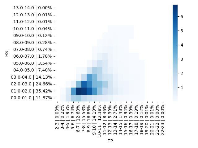
Create scatter Hs-Tp diagram:
tables.scatter_diagram(ds, var1='HS',
                       step_var1=1,
                       var2='TP',
                       step_var2=1,
                       output_file='Hs_Tp_scatter.csv')
HS/TP |
2-3 | 0.00% |
3-4 | 0.21% |
4-5 | 1.96% |
5-6 | 6.74% |
6-7 | 12.62% |
7-8 | 15.56% |
8-9 | 16.86% |
9-10 | 14.14% |
10-11 | 12.11% |
11-12 | 8.53% |
12-13 | 5.42% |
13-14 | 2.69% |
14-15 | 1.52% |
15-16 | 0.93% |
16-17 | 0.39% |
17-18 | 0.18% |
18-19 | 0.12% |
19-20 | 0.01% |
20-21 | 0.01% |
21-22 | 0.00% |
22-23 | 0.00% |
|---|---|---|---|---|---|---|---|---|---|---|---|---|---|---|---|---|---|---|---|---|---|
13.0-14.0 | 0.00% |
0.0 |
0.0 |
0.0 |
0.0 |
0.0 |
0.0 |
0.0 |
0.0 |
0.0 |
0.0 |
0.0 |
0.0 |
0.0 |
0.0 |
0.0 |
0.0 |
0.0 |
0.0 |
0.0 |
0.0 |
0.0 |
12.0-13.0 | 0.01% |
0.0 |
0.0 |
0.0 |
0.0 |
0.0 |
0.0 |
0.0 |
0.0 |
0.0 |
0.0 |
0.0 |
0.0 |
0.0 |
0.0 |
0.0 |
0.0 |
0.0 |
0.0 |
0.0 |
0.0 |
0.0 |
11.0-12.0 | 0.01% |
0.0 |
0.0 |
0.0 |
0.0 |
0.0 |
0.0 |
0.0 |
0.0 |
0.0 |
0.0 |
0.0 |
0.0 |
0.0 |
0.0 |
0.0 |
0.0 |
0.0 |
0.0 |
0.0 |
0.0 |
0.0 |
10.0-11.0 | 0.04% |
0.0 |
0.0 |
0.0 |
0.0 |
0.0 |
0.0 |
0.0 |
0.0 |
0.0 |
0.0 |
0.01 |
0.01 |
0.01 |
0.01 |
0.0 |
0.0 |
0.0 |
0.0 |
0.0 |
0.0 |
0.0 |
09.0-10.0 | 0.12% |
0.0 |
0.0 |
0.0 |
0.0 |
0.0 |
0.0 |
0.0 |
0.0 |
0.0 |
0.01 |
0.03 |
0.04 |
0.02 |
0.01 |
0.01 |
0.0 |
0.0 |
0.0 |
0.0 |
0.0 |
0.0 |
08.0-09.0 | 0.28% |
0.0 |
0.0 |
0.0 |
0.0 |
0.0 |
0.0 |
0.0 |
0.0 |
0.01 |
0.05 |
0.11 |
0.07 |
0.02 |
0.02 |
0.0 |
0.0 |
0.0 |
0.0 |
0.0 |
0.0 |
0.0 |
07.0-08.0 | 0.74% |
0.0 |
0.0 |
0.0 |
0.0 |
0.0 |
0.0 |
0.0 |
0.0 |
0.07 |
0.23 |
0.26 |
0.11 |
0.04 |
0.02 |
0.0 |
0.0 |
0.0 |
0.0 |
0.0 |
0.0 |
0.0 |
06.0-07.0 | 1.78% |
0.0 |
0.0 |
0.0 |
0.0 |
0.0 |
0.0 |
0.0 |
0.09 |
0.39 |
0.71 |
0.36 |
0.13 |
0.06 |
0.04 |
0.01 |
0.01 |
0.0 |
0.0 |
0.0 |
0.0 |
0.0 |
05.0-06.0 | 3.54% |
0.0 |
0.0 |
0.0 |
0.0 |
0.0 |
0.0 |
0.11 |
0.59 |
1.27 |
0.9 |
0.33 |
0.15 |
0.09 |
0.06 |
0.02 |
0.01 |
0.01 |
0.0 |
0.0 |
0.0 |
0.0 |
04.0-05.0 | 7.40% |
0.0 |
0.0 |
0.0 |
0.0 |
0.0 |
0.08 |
1.14 |
2.23 |
1.94 |
0.9 |
0.51 |
0.3 |
0.14 |
0.09 |
0.03 |
0.02 |
0.01 |
0.0 |
0.0 |
0.0 |
0.0 |
03.0-04.0 | 14.13% |
0.0 |
0.0 |
0.0 |
0.0 |
0.26 |
1.65 |
3.97 |
3.08 |
1.87 |
1.3 |
1.02 |
0.46 |
0.23 |
0.14 |
0.07 |
0.04 |
0.02 |
0.0 |
0.0 |
0.0 |
0.0 |
02.0-03.0 | 24.66% |
0.0 |
0.0 |
0.01 |
0.41 |
3.14 |
5.47 |
4.62 |
3.11 |
3.02 |
2.29 |
1.21 |
0.55 |
0.38 |
0.24 |
0.12 |
0.05 |
0.04 |
0.0 |
0.0 |
0.0 |
0.0 |
01.0-02.0 | 35.42% |
0.0 |
0.03 |
0.92 |
4.09 |
6.78 |
6.61 |
5.8 |
4.11 |
2.76 |
1.56 |
1.19 |
0.73 |
0.41 |
0.25 |
0.09 |
0.04 |
0.02 |
0.0 |
0.0 |
0.0 |
0.0 |
00.0-01.0 | 11.87% |
0.0 |
0.18 |
1.03 |
2.23 |
2.43 |
1.74 |
1.23 |
0.94 |
0.76 |
0.58 |
0.38 |
0.15 |
0.1 |
0.06 |
0.03 |
0.01 |
0.01 |
0.0 |
0.0 |
0.0 |
0.0 |
tables.scatter_diagram(ds, var1='HS',
                       step_var1=1,
                       var2='TP',
                       step_var2=1,
                       output_file='Hs_Tp_scatter.png')
Create table with monthly percentiles:
general_stats.table_monthly_percentile(data=ts.data, var='hs', output_file='hs_monthly_perc.csv')
Month |
5% |
50% |
Mean |
95% |
99% |
|---|---|---|---|---|---|
jan |
0.5 |
1.3 |
1.4 |
2.7 |
3.7 |
feb |
0.4 |
1.2 |
1.4 |
2.8 |
3.8 |
mar |
0.4 |
1.1 |
1.2 |
2.5 |
3.4 |
apr |
0.3 |
0.9 |
1.0 |
2.1 |
3.2 |
mai |
0.3 |
0.9 |
0.9 |
1.9 |
2.5 |
jun |
0.3 |
0.7 |
0.8 |
1.7 |
2.5 |
jul |
0.2 |
0.7 |
0.8 |
1.6 |
2.2 |
aug |
0.3 |
0.7 |
0.8 |
1.8 |
2.5 |
sep |
0.3 |
0.9 |
1.1 |
2.3 |
3.2 |
okt |
0.4 |
1.2 |
1.3 |
2.5 |
3.2 |
nov |
0.5 |
1.3 |
1.4 |
2.7 |
3.6 |
des |
0.4 |
1.3 |
1.4 |
2.8 |
3.5 |
Annual |
0.4 |
1.3 |
1.4 |
2.8 |
3.5 |
Create table with monthly min, mean, and max based on monthly values:
general_stats.table_monthly_min_mean_max(data=ts.data, var='hs',output_file='hs_montly_min_mean_max.csv')
Month |
Minimum |
Mean |
Maximum |
|---|---|---|---|
jan |
2.4 |
3.7 |
5.13 |
feb |
2.62 |
3.7 |
5.53 |
mar |
2.02 |
3.3 |
4.52 |
apr |
1.95 |
3.0 |
4.67 |
mai |
1.6 |
2.5 |
3.29 |
jun |
1.46 |
2.4 |
3.32 |
jul |
1.29 |
2.2 |
3.57 |
aug |
1.7 |
2.5 |
4.42 |
sep |
1.8 |
3.0 |
5.61 |
okt |
2.04 |
3.2 |
4.43 |
nov |
2.3 |
3.7 |
5.48 |
des |
2.46 |
3.6 |
5.14 |
Annual |
3.63 |
4.6 |
5.61 |
Create table with sorted statistics by Hs:
general_stats.table_var_sorted_by_hs(data=ts.data, var='tp', var_hs='hs', output_file='tp_sorted_by_hs.csv')
Hs |
Entries |
Min |
5% |
Mean |
95% |
Max |
|---|---|---|---|---|---|---|
0-1 |
140613 |
1.8 |
3.2 |
6.0 |
11.2 |
21.8 |
1-2 |
111055 |
3.6 |
4.3 |
6.8 |
12.3 |
21.8 |
2-3 |
24175 |
4.7 |
5.7 |
7.8 |
12.3 |
18.0 |
3-4 |
4058 |
6.3 |
6.9 |
9.8 |
13.5 |
18.0 |
4-5 |
571 |
7.6 |
9.2 |
11.6 |
14.9 |
18.0 |
5-6 |
40 |
9.2 |
10.2 |
11.8 |
14.9 |
14.9 |
6-7 |
0 |
|||||
0-7 |
280512 |
1.8 |
3.6 |
6.5 |
11.2 |
21.8 |
Directional Statistics
To generate directional stastistics, import dir_stats module:
from metocean_stats.stats import dir_stats
Create rose for overall data (method=’overall’) or for each month (method=’monthly’):
dir_stats.var_rose(ts.data, 'thq','hs','waverose.png',method='overall')

dir_stats.var_rose(ts.data, 'thq','hs','waverose.png',method='monthly')

Create table with min, mean, and maximum values as a function direction:
dir_stats.directional_min_mean_max(ts.data,'thq','hs','hs_dir_min_mean_max.csv')
Direction |
Minimum |
Mean |
Maximum |
|---|---|---|---|
345-15 |
2.2 |
2.8 |
3.7 |
15-45 |
2.2 |
3.0 |
4.0 |
45-75 |
2.4 |
3.3 |
4.3 |
75-105 |
2.5 |
3.3 |
4.1 |
105-135 |
2.3 |
3.4 |
4.2 |
135-165 |
2.8 |
4.1 |
5.5 |
165-195 |
3.0 |
4.2 |
5.6 |
195-225 |
1.9 |
3.4 |
5.5 |
225-255 |
1.9 |
3.1 |
4.8 |
255-285 |
2.0 |
2.9 |
4.4 |
285-315 |
2.0 |
2.7 |
4.2 |
315-345 |
2.0 |
2.9 |
4.1 |
Annual |
3.6 |
4.6 |
5.6 |
Extreme Statistics
To generate extreme stastistics, import extreme_stats module:
from metocean_stats import plots, tables
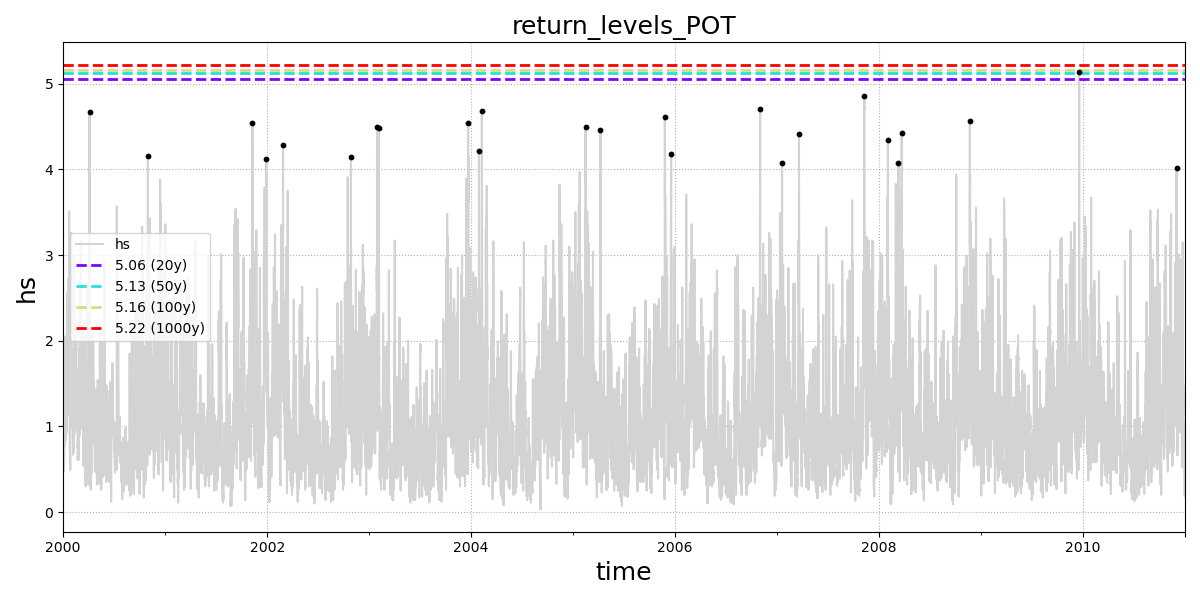
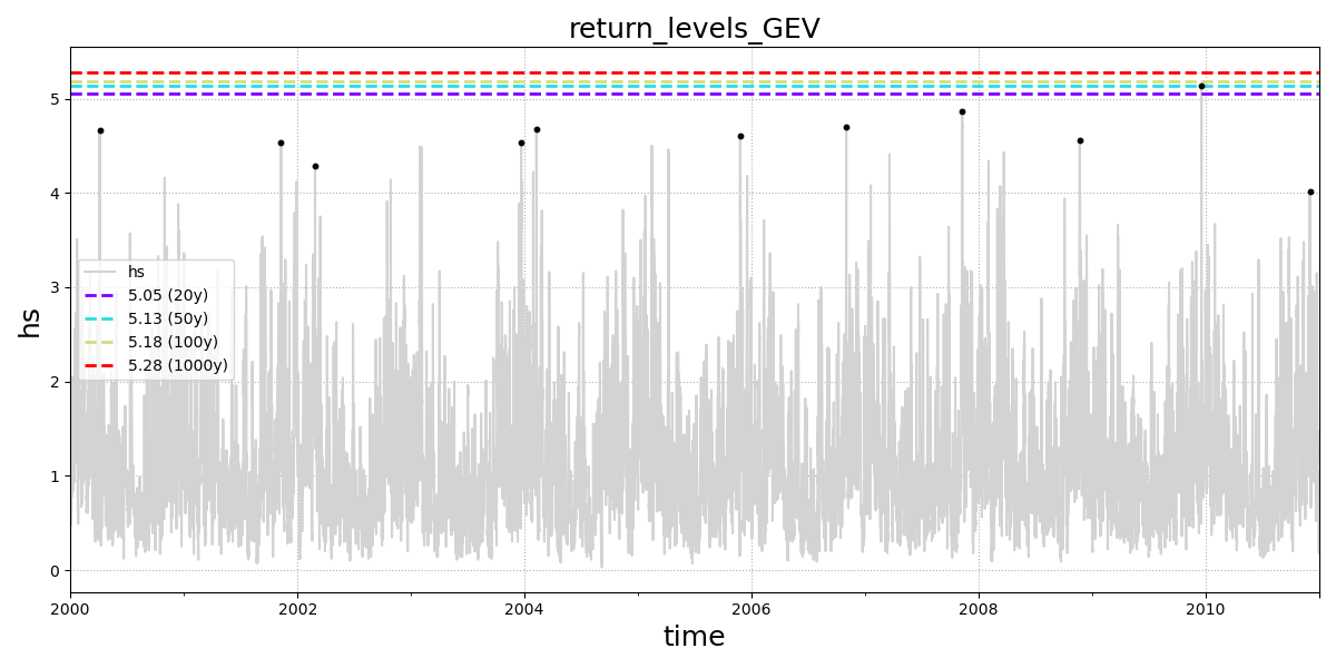
Create time series of Hs with return levels using POT and Annual Maximum(GEV):
rl_pot = extreme_stats.return_levels_pot(data=ds.data, var='hs',
         periods=[20,50,100,1000],
         output_file='return_levels_POT.png')
rl_am = extreme_stats.return_levels_annual_max(data=ds.data,
                                               var='hs',
                                               periods=[20,50,100,1000],method='GEV',
                                               output_file='return_levels_GEV.png')
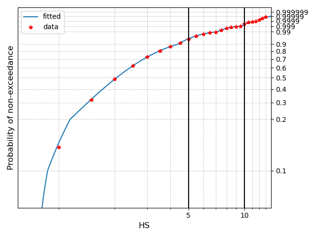
plots.plot_prob_non_exceedance_fitted_3p_weibull(ds,
                                                 var='HS',
                                                 output_file='prob_non_exceedance_fitted_3p_weibull.png')
Plot joint Hs-Tp contours for different return periods:
plots.plot_joint_distribution_Hs_Tp(ds,var_hs='HS',
                                    var_tp='TP',
                                    periods=[1,10,100,1000],
                                    title='Hs-Tp joint distribution',
                                    output_file='Hs.Tp.joint.distribution.png',
                                    density_plot=True)

Profile Statistics
To generate profile stastistics, import profile_stats module:
from metocean_stats.stats import profile_stats
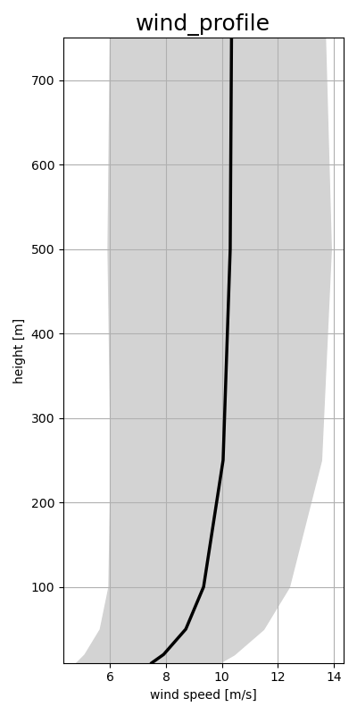
Estimate and plot mean wind profile with percentiles in shaded region:
mean_prof = profile_stats.mean_profile(data = ds.data, vars =
             ['wind_speed_10m','wind_speed_20m','wind_speed_50m',
             'wind_speed_100m','wind_speed_250m','wind_speed_500m',
             'wind_speed_750m'],
             height_levels=[10,20,50,100,250,500,750],
             perc=[25,75],
             output_file='wind_profile.png')
Calculate the wind speed shear over any two heights of the input profile and plot in a histogram and output shear values. Percentiles are shown as shaded region.: .. code-block:: python
- profile_stats.profile_shear(data = ds.data, vars =
[‘wind_speed_10m’,’wind_speed_20m’,’wind_speed_50m’, ‘wind_speed_100m’,’wind_speed_250m’,’wind_speed_500m’, ‘wind_speed_750m’], height_levels=[10,20,50,100,250,500,750], z=[20,250], perc = [25,75], output_file=’wind_profile_shear.png’)

Map Statistics
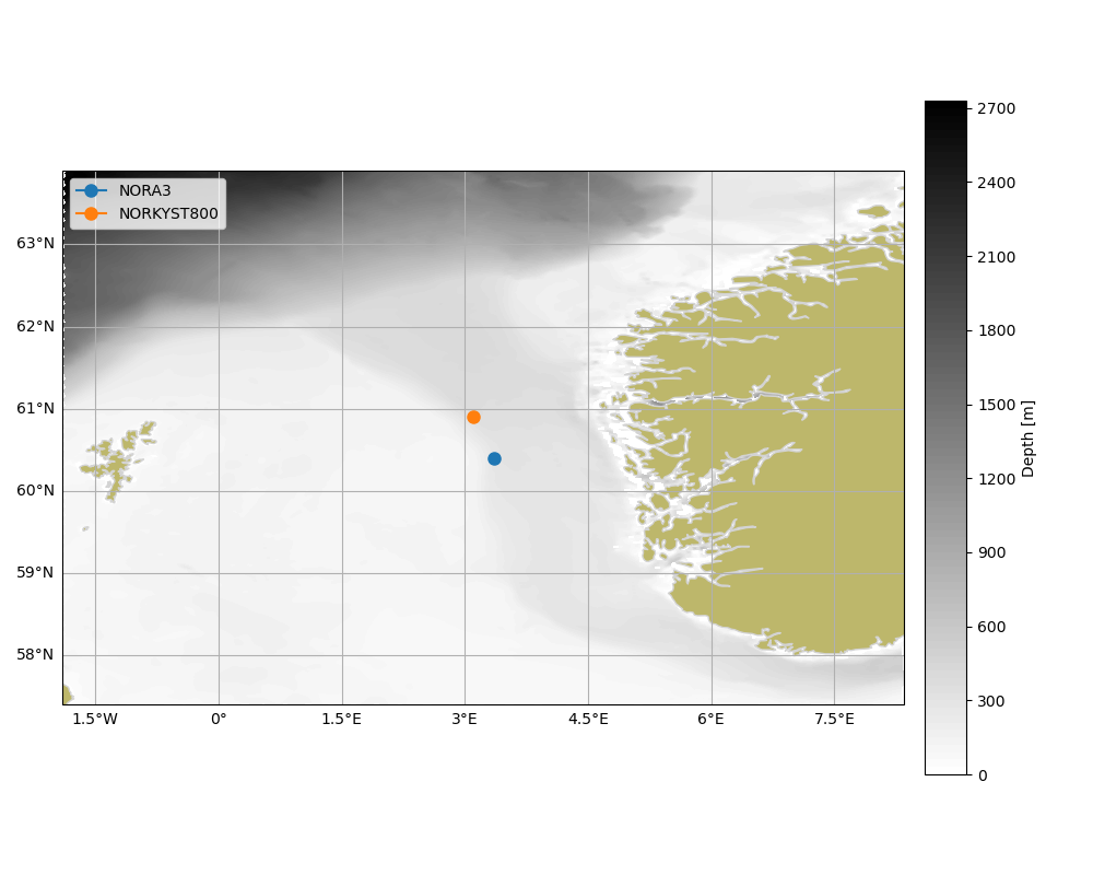
Plotting maps:
from metocean_stats.stats.map_funcs import *
Plot map with points of interest:
plot_points_on_map(lon=[3.35,3.10],
                   lat=[60.40,60.90],
                   label=['NORA3','NORKYST800'],
                   bathymetry='NORA3')
Plot extreme signigicant wave height based on NORA3 data:
plot_extreme_wave_map(return_level=50,
                      product='NORA3',
                      title='50-yr return values Hs (NORA3)',
                      set_extent = [0,30,52,73])

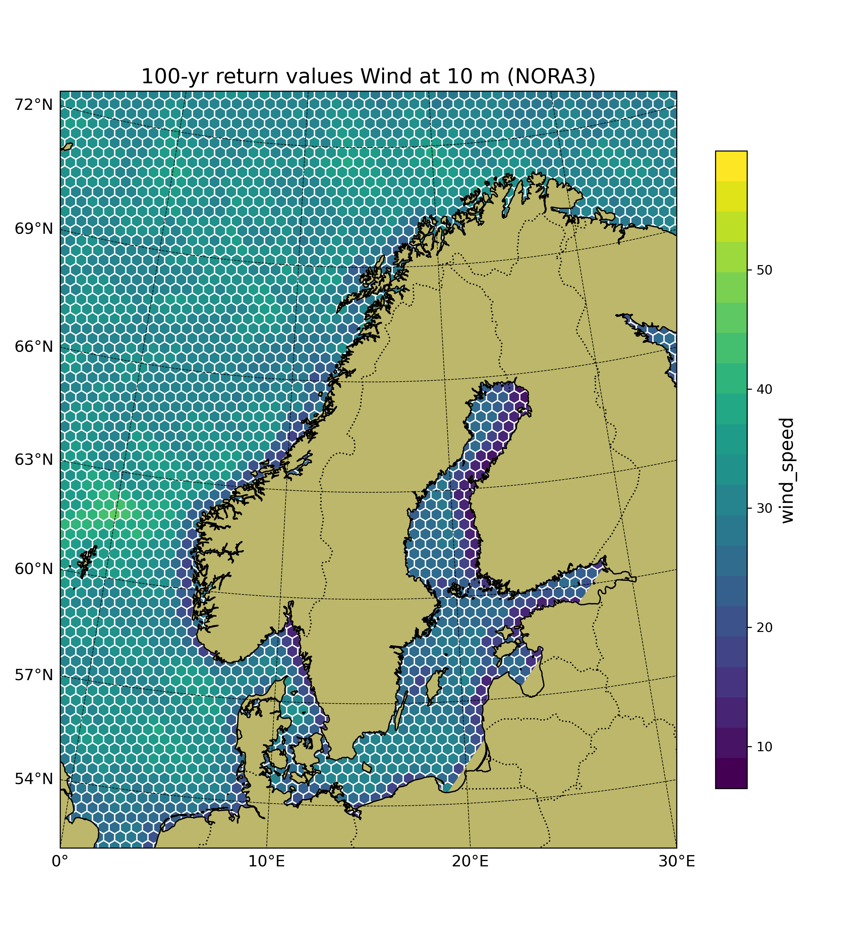
Plot extreme wind at 10 m height based on NORA3 data:
plot_extreme_wind_map(return_level=100,
                      product='NORA3',
                      level=0,
                      title='100-yr return values Wind at 10 m (NORA3)',
                      set_extent = [0,30,52,73])